In Part 1 of this series, I wrote about the concept of measurement. We saw how measurement is not about capturing real-world observations as a single value but rather about reducing our uncertainty about the range of possible values.
In Part 2, we discussed how we can take “intangible” things like “employee empowerment,” and bring that into a space that can be measured numerically.
For the finale, I want to give you the tools you need to quantify your uncertainty for most of your day-to-day measurement needs. By the end of this read, you’ll have what you need to effortlessly determine the potential range of values for any given measurement based on your data.
Math-less Median
Imagine you’re trying to predict the number of widgets you can sell per day. You can rephrase this mathematically to ask “What is the median number of widgets that I would sell per day if I took a really large sample”?
However, it would take a long time to generate a “large sample.” Luckily, you don’t need to!
You measure widgets sold for 5 days and come up with the following set:
Day 1 – 5
Day 2 – 10
Day 3 – 7
Day 4 – 15
Day 5 – 3
You can sort the numbers in order:
3, 5, 7, 10, 12
You can be 93.8% sure that the median number of widgets sold per day will be between 3 (the smallest value) and 12 (the largest value).
If you had additional data (new data bolded), say:
3, 5, 6, 7, 7, 9, 10, 12
You can simply take the second smallest and largest values and have 93% confidence that the median is between 5 and 10 (Notice the tighter range).
In general, you depending on your sample size, you can use the nth smallest and largest values from the table below to identify a narrower range on the median value for the population you’re sampling from.
| Sample Size | nth Largest & Smallest Values | Confidence |
|---|---|---|
| 5 | 1st | 93.8% |
| 8 | 2nd | 93% |
| 11 | 3rd | 93.5% |
| 13 | 4th | 90.8% |
| 16 | 5th | 92.3% |
| 18 | 6th | 90.4% |
| 21 | 7th | 92.2% |
| 23 | 8th | 90.7% |
| 26 | 9th | 92.4% |
| 28 | 10th | 91.3% |
| 30 | 11th | 90.1% |
This can be a very practical way to quickly understand the level of confidence you can have in your collected data. Note that this will hold true regardless of the distribution of your data!
This method was popularized by Doug Hubbard and is known as the “Mathless Table.” I’ve previously written about how and why this works if you’re curious.
Small Samples, Sound Statistics
Many phenomena in our world are approximately normally distributed, with more observations near the mean (average) and fewer observations the further away from the mean you go.
Some examples include shoe sizes, students’ averages, and heights of individuals.
When you’re measuring something with this characteristic and you don’t know the variance for the underlying population your data came from, you can use the T-distribution to estimate the population mean!
The T-distribution is particularly useful when dealing with small samples, as it adjusts for the increased uncertainty.
Let’s work through a real-world example using simple excel formulas:
Let’s say you produce bricks for buildings, and you want to know the average force that your bricks can withstand without breaking for each batch you produce.
One way to measure that would be to break all your bricks and take the average of the force applied to break them.
But that would mean you won’t have a brick business anymore!
T-distribution to the rescue!
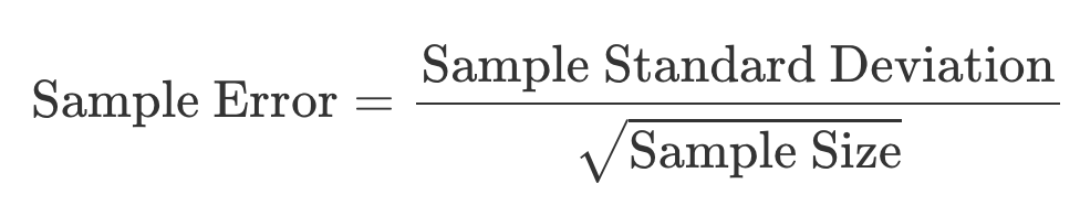
You jot down the Breaking Force (in N/mm²) for a handful of bricks:
It’s very easy to take this data and calculate our uncertainty around the population mean in a few simple steps!
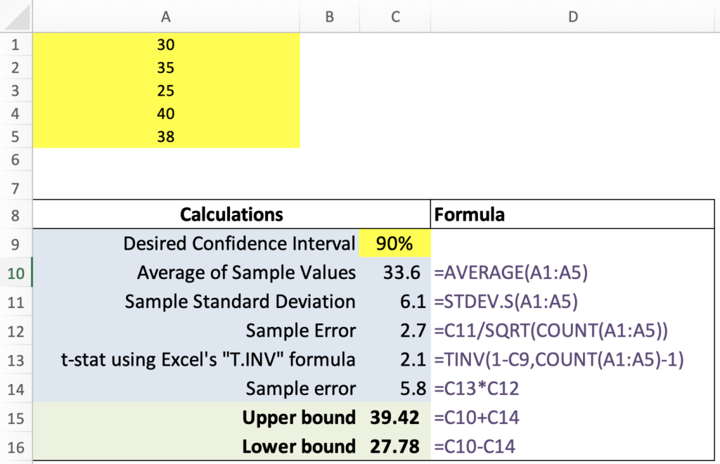
Step 1: Calculate the Sample Mean and Sample Standard Deviation.
Using Excel:
- Mean:
=AVERAGE(A1:A5)results in 33.6 N/mm² - Sample Standard Deviation:
=STDEV.S(A1:A5)gives 6.11 N/mm²
Step 2: Determine the Degrees of Freedom. Think of this as the number of values free to vary in the sample. It’s computed as the sample size minus one.
Using Excel:
- Sample Size:
=COUNT(A1:A5)which equals 5 - Degrees of Freedom:
=5-1giving a result of 4
Step 3: Compute the Sample Error. It tells us how much our sample mean might differ from the true population mean.
Formula:
For our data, SE is approximately 2.73 N/mm².
Step 4: Calculate the t-value for the Confidence Interval.
For a 90% confidence interval, we’ll need the critical t-values. These values indicate how many standard errors to add and subtract from our sample mean to determine the interval.
Using Excel:
- t-value:
=TINV(0.10, 4)which equals 2.13
This t-value will be used for both the upper and lower bounds. Note that we’re inputting 0.10 (which is 1 – 0.9) for the 90% confidence interval, and this is independent of your data.
Step 5: Determine the Confidence Interval (CI) bounds.
Using the t-value:
- CI Lower Bound:
Sample Mean - (t-value × Sample Error)= 27.78 - CI Upper Bound:
Sample Mean + (t-value × Sample Error)= 39.42
We can be 90% certain that the true population mean lies within this interval. This provides us with a statistical foundation to make informed decisions about the average breaking force of our bricks.
That’s it! You can see how it all fits together in Excel in the image below.
Precisely Predicting Proportions
Have you ever wondered how to measure things like the success rate of a new marketing campaign, or perhaps the likelihood of rain tomorrow? When dealing with proportions or probabilities of hit or miss events, the Beta distribution is your best friend.
Imagine you’ve been burning the midnight oil at your tech startup. After several brainstorming sessions, you’ve conceived a potentially revolutionary feature. However, for this feature to be commercially viable, at least 60% of your user base must love it.
You, being data-savvy product manager, decide that before diving head-first into a full launch, you can test the waters with a scaled down version of the solution with a handful of your users before investing the big dollars to build it out fully. If, given the experiment results, there’s at least an 85% chance that the approval rate is 60% or higher (for your broader user-base), then you’ll go forward to build the feature. Note that there’s nothing special about the 85% chance. It’s simply a matter of specifying your risk tolerance.
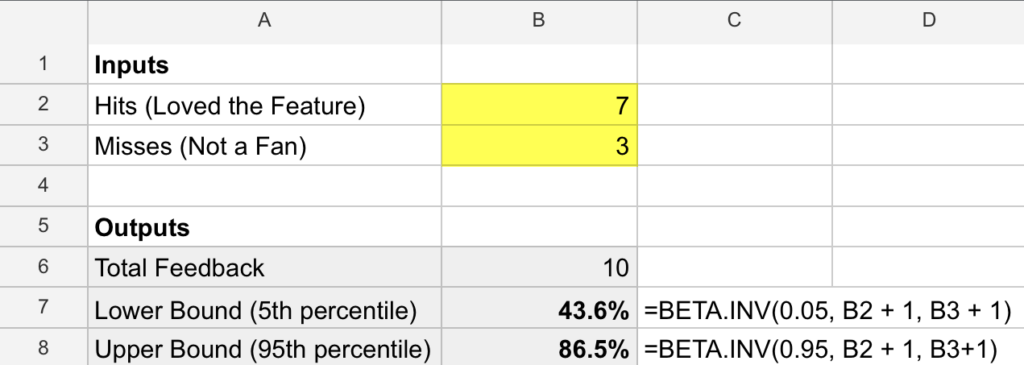
From an initial 10 users: 7 are all praises, while 3 have reservations. That’s a 70% approval rate. But can such a tiny sample give you the confidence to meet that crucial 85% probability?
Time to delve into the Beta distribution!
Round 1: The Initial Test
Given a number of positive responses (hits) and negative responses (misses), the Beta distribution can help us understand how wide our uncertainty around the true proportion in a population is based on a sample.
In Excel, you can use the BETA.INV function with three parameters: the desired confidence level (like the 5th or 95th percentile), hits + 1, and misses + 1. This function then calculates the estimated approval rate for that confidence level, providing insights into potential outcomes for the entire population.
It helps to visualize the probability density curve for the distribution which clearly highlights all the possible values the real population’s approval rate may take based on the information provided from the sample, and how likely each value is. The values that are higher on the y-axis are more likely.
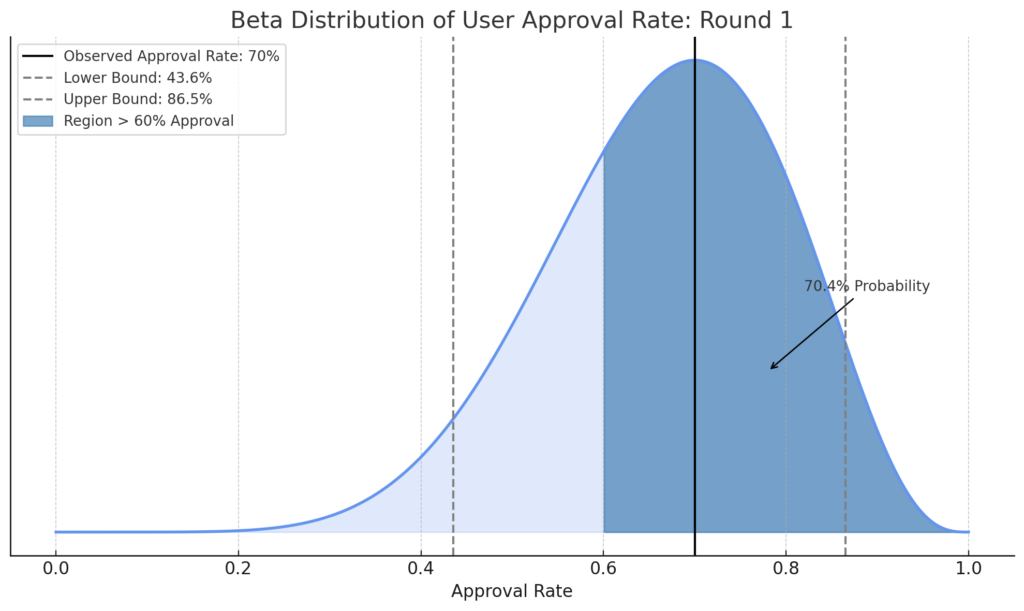
By computing the area for the region under the curve for any segment on the x-axis, you can figure out what the probability of falling within that region is. Although your observed approval rate (70%) meets the threshold, there’s still only a 70.4% chance the real underlying proportion is above 60%! That means there’s a 29.6% chance of not meeting the bar!
Recalling that your requirement was at least an 85% chance of being above a 60% approval rate, you decide that the stakes are too high to move forward given this evidence, and it’s worth extending your experiment to collect more data and reduce uncertainty (in effect, narrowing down the possible outcomes).
Round 2: The Extended Test
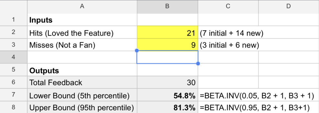
You collect feedback from 20 more users. This time, 14 applaud, but 6 aren’t convinced.
Updating your Excel sheet:
Let’s visualize our uncertainty now, after the 2nd round.
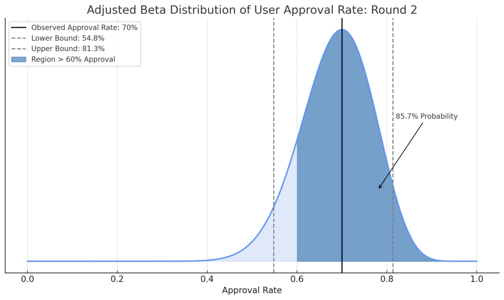
You see that even though the observed approval rate remained 70%, with the additional feedback your uncertainty around the possible true value of your population has been greatly reduced (i.e. the probability distribution is now tighter).
You calculate the probability that the approval rate exceeds 60% by taking the area under the graph (1 - BETA.DIST(0.6, B2+1, B3+1, TRUE)) and eureka! Sitting at 85.7%, it just surpasses the 85% threshold, giving you the confidence to move forward.
Balancing Beliefs and Bits
Decision-making in business often hinges on assessing probabilities. Bayes’ theorem provides a structured approach, allowing companies to adjust their predictions by integrating new evidence, ensuring that decisions are not just data-driven, but dynamically updated with fresh insights.
Imagine you’re a series A stage venture capitalist on the hunt for the next unicorn (a company with a $1B+ valuation). You know that only 2% of startups ever make it make it there. Additionally, of all the unicorns out there, 20% secured funding from a top-tier VC. You also know that only 10% of all startups manage to work with these top VCs. [Note: these numbers are completely made up]
The next day, you stumble upon a fast-growing startup, who’s seed round was backed by some of the most reputable VCs in the industry. Your question is:
What’s the chance that this startup will become a unicorn given they’re backed by top-tier VCs?
At first glance, you’re tempted to say 20%, but you get this nagging feeling that you’re missing something… You know that 20% of the unicorns were funded by top VCs, but here we’re flipping the question… You vaguely remember something you learned in statistics class, so at the risk of triggering your PTSD (Post-Traumatic Statistics Disorder), you open your dusty old textbook to find Bayes’ theorem:
\[ P(A|B) = \frac{P(B|A) \times P(A)}{P(B)} \]
Where:
- \(P(A|B)\) is the probability of event \(A\) happening given that \(B\) has happened.
- \(P(B|A)\) is the probability of event \(B\) happening given that \(A\) has occurred.
- \(P(A)\) and \(P(B)\) are the probabilities of events \(A\) and \(B\) happening overall, respectively.
“Easy enough,” you think to yourself, and define the inputs to be relevant to your case.
- \(A\) is the event of a startup becoming a unicorn.
- \(B\) is the event of a startup getting funded by a top-tier VC.
Given our data:
\(P(A) = 2\%\) chance of a random startup becoming a unicorn
\(P(B|A) = 20\%\) chance of having have received seed funding from a top VC given that they are a unicorn
\(P(B) = 10\%\) chance of a startup getting seed funding by a top VC
Plug these values into our formula, and voilà! You can now easily calculate the probability of a startup becoming a unicorn given they‘ve raised a seed round from a top VC.
\[
P(A|B) = \frac{\stackrel{0.20}{P(B|A)} \times \stackrel{0.02}{P(A)}}{\stackrel{0.10}{P(B)}} = 0.04
\]
You’re surprised to see the results! 4% is a far cry from the intuitive 20% you originally thought it would be. With this new knowledge in hand, you decide to place less of an emphasis on their VC partners on the seed round and focus on deeper due diligence.
While I covered a basic example here, Bayes’ theorem offers a powerful lens to refine decisions as new data emerges. From market forecasting to customer insights, it’s a game-changer, turning uncertainties into strategic advantages.
If you want to gain a deeper intuition for why Bayes’ formula is structured as it is, this video from 3blue1brown has some of the best visualizations I’ve seen on the topic. If you want to take it to the next level and apply advanced Bayesian methods in your analysis, Richard McElreath’s Statistical Rethinking lectures on Youtube are pure gold.
Conclusion
Diving into the world of statistics and measurement can often feel like navigating a dense forest. Yet, as we’ve seen, with the right tools and methodologies, we can make precise decisions even when faced with uncertainty.
Whether you’re estimating median values with limited data, gauging the potential of a startup, or predicting market trends using Bayesian thinking, the key is to embrace the uncertainty and use it to your advantage.
As we conclude this series, remember that in the realm of data, it’s not just about the numbers we have but understanding and quantifying what lies between them. Until next time, keep measuring, keep questioning, and most importantly, keep learning!