Too often in business, we ignore measurements with small sample sizes because they are not “statistically significant,” but rarely, if ever, do we actually do the math to support that decision!
The fact is that it is precisely when we are highly uncertain about something that any data will greatly reduce our uncertainty.
I’m going to play out 2 scenarios from a fantastic book called “How to Measure Anything” by Douglas Hubbard so you can experience the “Aha!” moment for yourself.
By the end of this blog post, you’ll have an understanding of situations where small data can tell you a lot, and you will think twice before dismissing precious information about your business.
The Rule of 5
Imagine you’re the IT manager for a company with 100,000 employees, and you’re thinking of deploying software that will automate some routine tasks like filing expense reports.
You’ve put together an ROI model for the project. Still, to know if this project will save more money than you pay for it, you need to gather data about the median time employees spend on this task today (that is, the number that evenly splits the employees by the number of minutes spent on this task).
How would you go about collecting this data?
Surveying all 100,000 employees would be unreasonable due to high costs. How big of a sample do you really need to answer this question?
What if I told you that a sample of 5 might be enough to validate your model?
Let’s say you randomly pick 5 people from the company and ask them how long they spend on this task every month.
Their responses are 15, 18, 20, 27 and 30 minutes.
Is this information enough? Most would say no, but let’s dig into this.
What are the chances that the true median time spent by employees falls between the lowest (15) and highest (30) values seen in your 5-person survey?
Doing the math, it can be calculated that the probability that the median is between 15 and 30 minutes is a whopping 93.75%.
You might say this is a wide range, but maybe before measuring, you thought it was 8 minutes or 1 hour. In fact, if all you needed for the project to break even was employees spending more than 10 minutes on this task, you could fairly confidently go ahead with the project. Conversely, if your breakeven point is 1 hour, you can confidently reject the project.
The same rule applies to any population with any distribution and can be extended if you have more than 5 data points. If we have more data, we can actually get a tighter bound than the min and max of our samples. Depending on your sample size, you can take the nth smallest and largest values in your sample instead.
| Sample Size | nth Largest & Smallest Values | Confidence |
|---|---|---|
| 5 | 1st | 93.8% |
| 8 | 2nd | 93% |
| 11 | 3rd | 93.5% |
| 13 | 4th | 90.8% |
| 16 | 5th | 92.3% |
| 18 | 6th | 90.4% |
| 21 | 7th | 92.2% |
| 23 | 8th | 90.7% |
Derivation (Optional)
By definition, the probability of a value being above or below the median is 50%. For the population median to not be between the min and max of your sample, you’d have to get 5 samples in a row below the median OR 5 samples in a row above the median.
The probability this happening is (0.5)⁵ + (0.5)⁵= 0.0625, thus the probability of the inverse (the median being between the min and max of the sample) is 1 – 0.0625 = 0.9375
The Urn of Mystery
I want to make a bet with you.
I bring you into a factory that produces thousands of urns (vases) with a mix of black and white marbles in them. Each urn contains 10,000 marbles and the mixture percentage is completely random, with any ratio of white to black marbles from 0% to 100% being equally likely.
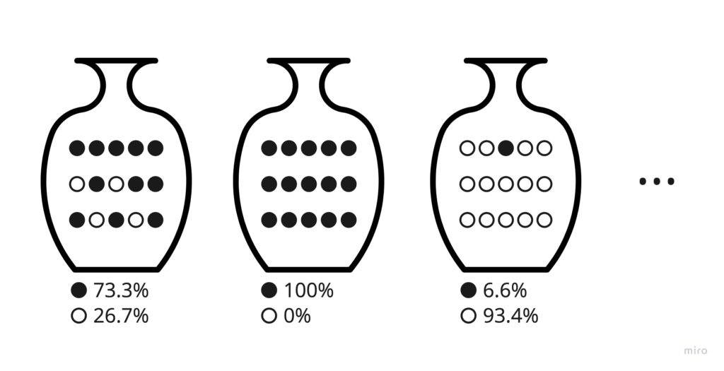
We’ll choose an urn at random, and I’ll try to guess the colour of the majority of the marbles in that urn. I’ll give you 2:1 odds, where if I get it right, you give me $5, but if I wrong, I give you $10. We’ll play for 100 rounds.
You know I have a 50-50 chance of guessing the right colour. You’re pretty savvy, so you can calculate your expected return per game.
Expected Winnings Per Game = (0.5 chance of losing ) (-$5) + (0.5 chance of winning) ($10) = $2.50
That means after 100 games, you’d end up with about $250 in your pocket. You will probably take this deal with a smile on your face!
“That’s hardly fair,” I say. “To give me more of a chance to win, will you let me take a look at the colour of a single randomly chosen marble out of each urn before making my guess?”
Assuming there’s no foul play at work here, would you still take this bet?
1 single sample is not going to change the expected outcome by much, right? Maybe the new chance of losing is 51% instead of 50%… You chuckle and say, “You’re on!”
100 games later, you’re writing me a nice $125 cheque.
What in the world just happened?
My strategy was simple. If I got a black marble, I guessed black, and if I got a white marble, I guessed white. This simple strategy boosted my chances of winning from 50% to an astonishing 75%!
When given the maximum uncertainty about some population proportion, there’s a 75% chance that any single sample is drawn from the majority group. This is formally known as the single sample majority rule.
Derivation (Optional)
I initially explained this phenomenon to myself by relying on the intuitive interpretation of the Beta distribution. The Beta distribution is defined over [0, 1], making it an ideal candidate to represent uncertainty about a population proportion (the percentage of a population matching some criteria).
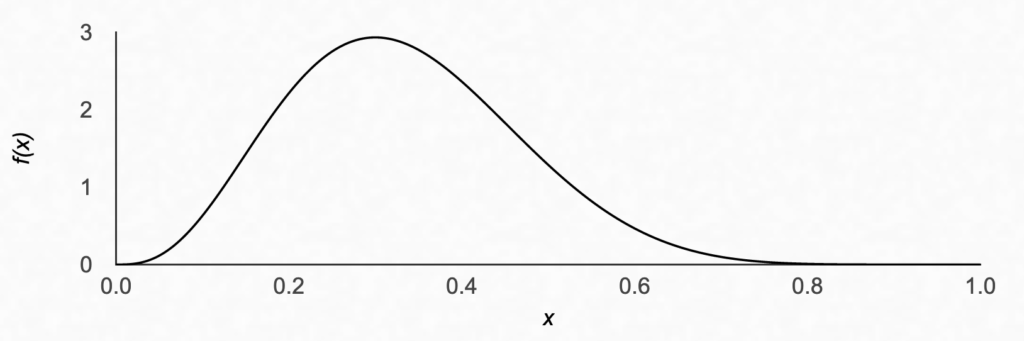
It parameterized by α and β greater than 0, which have this nifty property that for positive integer values of α and β, they can be interpreted as the α = # Hits + 1 and β = # Misses + 1. For example, if you’ve taken sample of 10 people and 3 people said they like ice cream, α = 3 + 1 = 4 and β = 7 + 1 = 8. The distribution for x, the percent of people who like ice cream, would look like this.
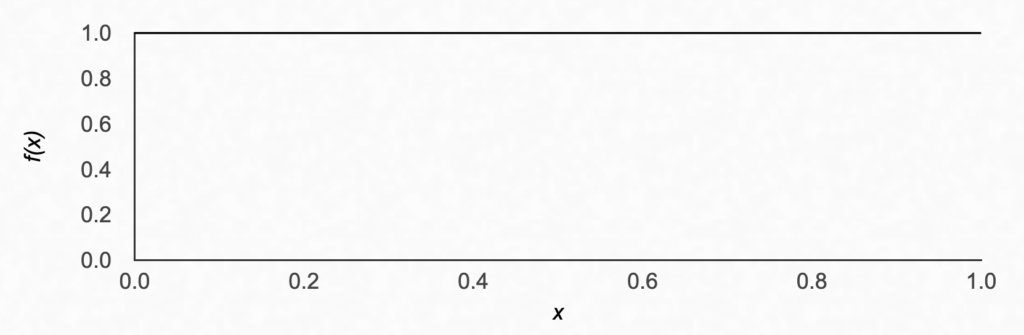
If you haven’t sampled yet, you have 0 hits and 0 misses, meaning α = 1 and β = 1. This means you don’t know anything about the population proportion, and you’ll get a uniform prior, meaning any value is equally likely.
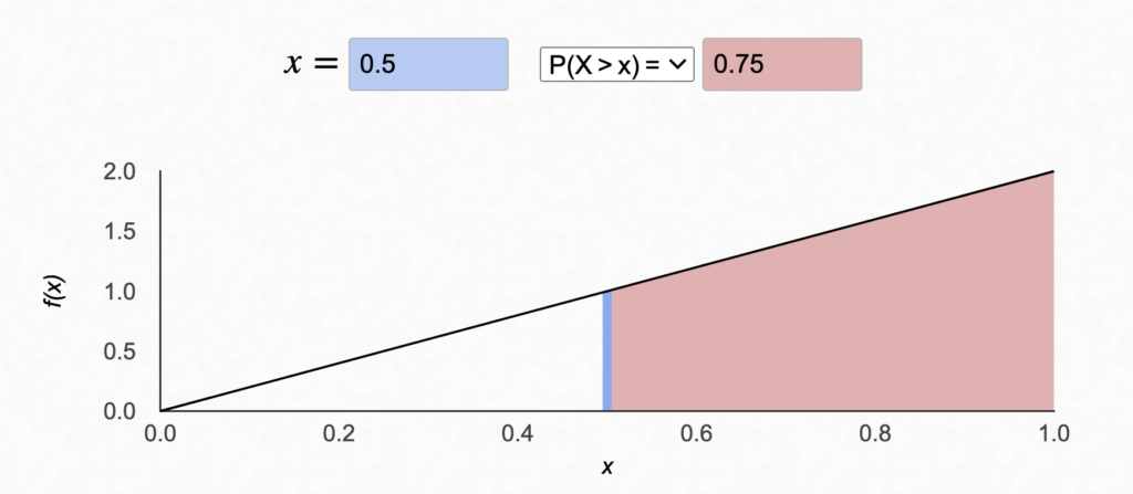
This is the situation we’re in with our marbles. We can frame the problem such that x is the ratio of the marbles in the urn having the same colour as the marble we sampled. By definition, the colour marble we sampled will be considered a “hit.”
Once we take our first sample, we can simply add 1 to our hits, and therefore add 1 to α. To get the probability that the marble is from the majority in the urn, we simply need to calculate P(x > 0.5). We can do this by calculating the area under the curve where x> 0.5.
This can also be done in excel with a simple formula:
= 1 - BETA.DIST(0.5, 2, 1, TRUE)The arguments to BETA.DIST are defined in the order x, α, β, cumulative, where cumulative=TRUE tells excel to calculate the area under the curve for values x < 0.5, which is why we’re subtracting it from 1.
The more mathematically rigorous explanation follows a similar path:
- Let θ be the proportion of black marbles in a given urn. Since we’re choosing an urn randomly, the probability of drawing black follows the uniform distribution which can also be represented using the Beta distribution ➡ P(θ) ~ Uniform(0,1) ~ Beta(α=1, β=1)
- The probability of drawing a black marble given θ follows the Bernoulli distribution ➡ P(Draw Black) ~ Bern(θ)
Using Bayes’ theorem, we know that
P(θ|Draw Black) ∝ P(Draw Black |θ) • P(θ)
The prior P(θ) is Beta distributed and P(Draw Black |θ) is Bernoulli distributed. Since the Beta distribution is the conjugate prior to the Bernoulli distribution, that implies the posterior probability P(θ|Draw Black) will also be Beta distributed.
In fact, through the magic of mathematical plug and chug, it can be derived that the posterior pdf will follow the distribution Beta(α+1, β) = Beta(2,1) if we draw a black marble and Beta(α, β+1) = Beta(1,2) if we draw a white marble. We can then use the CDF of the distribution to get to 0.75, as we did above.
WHY Small Samples Work
These two problems have something in common, which is the same thing that packs so much information into a few samples:
We knew nothing before we started measuring.
The amount a measurement reduces our uncertainty about a particular quantity is huge when we know little but fades as we get more data.
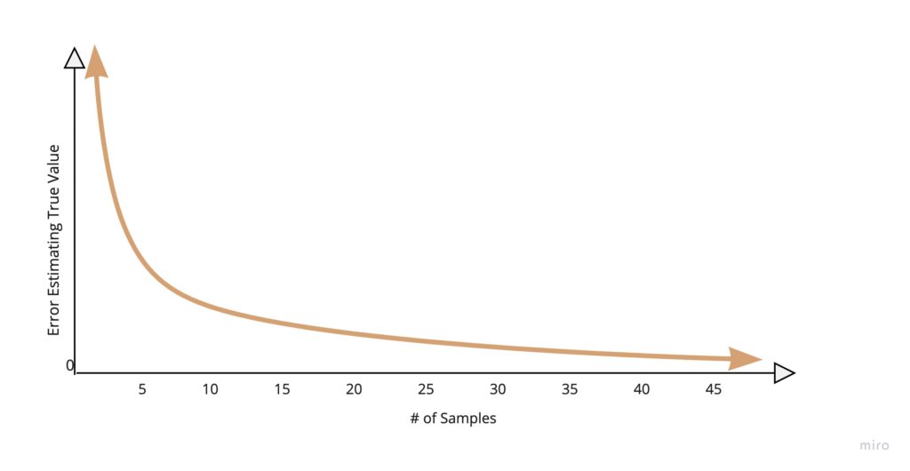
The first few samples reduce our potential range of answers by a significant margin, but beyond 30 samples, you’d need another 90 samples to cut your uncertainty in half.
WHEN Small Samples Work
An important thing to note here is is that the more homogenous your population, the faster your uncertainty will decrease. If you measure the weight of a penny, that first sample will tell you a lot!
If you measure something heterogenous like dollars spent at Walmart by customers per visit, it’s gonna take a lot longer to narrow the bands on your confidence intervals.
The key takeaway is that measurement is a process that reduces your uncertainty, and you only need to measure until you’re satisfied with the level of uncertainty and can make a decision.
In the Walmart example, if all you care about is having an average customer spend greater than $20 and after a sample of 7 customers, your 90% confidence interval is $100-$600 per customer, I would just call it a day and find something better to do with my time (like reading “How to Measure Anything”).
Conclusion
Next time you’re faced with a measurement challenge, keep the following principles in mind:
- Unless you’re doing some kind of hypothesis testing, you probably don’t need to worry about “statistically significant” results. This concept is often misremembered and misinterpreted. Even when it is interpreted correctly, it’s often not what the decision-maker wants to know.
- When you know nothing about the value of some quantity, even a few samples can help guide your decisions, as long as you’re aware of the range of uncertainty associated with the measurements. You can use the Rule of 5 or the Single Sample Majority Rule as a casual way to quantify that range.
- You only need to keep measuring until you’ve reduced uncertainty around a value enough to know whether it meets the threshold that has a bearing on your decision-making.