When I first started building the Data Vault at Georgian, I couldn’t decide what column data type to use as my tables’ primary key.
I had heard that integer joins vastly outperform string joins, and was worried about degrading join performance as our data grew.
In the SQL databases of the operational world, this decision is pretty much made for you by giving you auto-incrementing int primary keys out of the box.
In the Data Warehousing world, however, whether you’re building a Kimball or Data Vault or something else, you need to make this choice explicitly.
You can generate an integer, a UUID string, or hash your columns into a single column, which comes with many benefits. As if that wasn’t complex enough, your hashed keys can be stored as strings or bytes, and each algorithm’s output may vary in length.
This brings up a question:
How does the column type of keys affect the speed of joins in Data Warehouses?
After some digging, I found some benchmarks for transactional databases, but that’s not what I was looking for. Logically speaking, integers must be faster than strings and byte-strings because there are generally fewer bytes to scan. But… by how much!?
Knowing the answer seemed very important because, in a data warehouse, a bad choice can get multiplied a billion-fold.
I finally buckled under the pressure of curiosity and decided to run a benchmark on BigQuery to answer this question for myself.
Experiment Design
I decided to generate 5 million rows of random numbers and test joining them (without cache) on the following types of keys:
- sequential integer (1-5M)
- farm fingerprint hash integer
- MD5 as bytes
- MD5 as a string (hex-encoded)
- SHA1 as bytes
- SHA1 as a string (hex-encoded)
Here is the code I used to generate the tables I wanted to join:
/* GENERATE_ARRAY has a limit of 1M rows
   so I had to union a bunch of them together */

WITH
  keys_1 AS (SELECT * FROM UNNEST(GENERATE_ARRAY(1,1000000)) AS key),
  keys_2 AS (SELECT * FROM UNNEST(GENERATE_ARRAY(1000001,2000000)) AS key),
  keys_3 AS (SELECT * FROM UNNEST(GENERATE_ARRAY(2000001,3000000)) AS key),
  keys_4 AS (SELECT * FROM UNNEST(GENERATE_ARRAY(3000001,4000000)) AS key),
  keys_5 AS (SELECT * FROM UNNEST(GENERATE_ARRAY(4000001,5000000)) AS key),
  keys_union AS (
    SELECT key FROM keys_1 UNION ALL
    SELECT key FROM keys_2 UNION ALL
    SELECT key FROM keys_3 UNION ALL
    SELECT key FROM keys_4 UNION ALL
    SELECT key FROM keys_5
  ),
  keys_hashed AS (
    SELECT
      key,
      MD5(CAST(key AS STRING)) as key_md5_bytes,
      TO_HEX(MD5(CAST(key AS STRING))) as key_md5_str,
      FARM_FINGERPRINT(CAST(key AS STRING)) AS key_farm,
      SHA1(CAST(key AS STRING)) AS key_sha_bytes,
      TO_HEX(SHA1(CAST(key AS STRING))) AS key_sha_str
     FROM keys_union
  )
  SELECT *, rand() AS val FROM keys_hashed
And here is the code I used to test make join:
SELECT
  t1.val, t2.val
FROM bq_benchmark.t1
JOIN bq_benchmark.t2
USING(<key column here>);
I ran the join query 30 times for each key type to use a Z-test to test for the difference between the mean query times and get reliable confidence intervals.
Experiment Results
Some definitions you may find helpful when interpreting the results:
Lower Bound 90% Confidence Interval: There’s a 5% probability that the true mean query time is below this number.
Upper Bound 90% Confidence Interval: There’s a 5% probability that the true mean query time is Above this number.
Standard Deviation: A measure of how much deviation (on either side) from the mean query time we observed in our sample on average.
Standard Error of the Estimate of The Mean: How much the true mean query time deviates from the estimated mean query time of our sample.
| MB Processed | Lower Bound 90% CI (s) | Mean Query Time (s) | Upper Bound 90% CI (s) | Std. Dev | Std. Error of Estimate of Mean | |
|---|---|---|---|---|---|---|
| Int | 153 | 3.92 | 4.05 | 4.18 | 0.42 | 0.078 |
| Farm Int | 153 | 4.19 | 4.30 | 4.40 | 0.34 | 0.06 |
| MD5 Bytes | 248 | 4.40 | 4.57 | 5.90 | 0.56 | 0.10 |
| MD5 String | 400 | 4.74 | 6.09 | 6.28 | 0.63 | 0.12 |
| SHA1 Bytes | 286 | 4.61 | 4.77 | 4.94 | 0.55 | 0.10 |
| SHA1 String | 477 | 5.50 | 5.65 | 5.80 | 0.50 | 0.09 |
You may also care to have a comparative view of the above data. To keep things simple, I will only compare the difference in mean query times and ignore the confidence intervals of the differences (which I’ve made available in the excel download below).
| Base Type | Compared Type | Absolute Diff | Relative (1+ is Slower) | Confidence in Difference |
|---|---|---|---|---|
| Int | Farm | 0.24 s | 1.06ⅹ | 99.27% |
| MD5 Bytes | 0.52 s | 1.13ⅹ | 100% | |
| MD5 String | 2.03 s | 1.5ⅹ | 100% | |
| SHA1 Bytes | 0.72s | 1.18ⅹ | 100% | |
| SHA1 String | 1.59 s | 1.39ⅹ | 100% | |
| Farm | MD5 Bytes | 0.28 s | 1.06ⅹ | 98.96% |
| MD5 String | 1.79 s | 1.42ⅹ | 100% | |
| SHA1 Bytes | 0.48 s | 1.11ⅹ | 100% | |
| SHA1 String | 1.35 s | 1.31ⅹ | 100% | |
| MD5 Bytes | MD5 String | 1.51 s | 1.33ⅹ | 100% |
| SHA1 Bytes | 0.2 s | 1.03ⅹ | 91.93% | |
| SHA1 String | 1.07 s | 1.23ⅹ | 100% | |
| SHA1 Bytes | MD5 String | 1.31 s | 1.27ⅹ | 100% |
| SHA1 String | 0.87 s | 1.18ⅹ | 100% | |
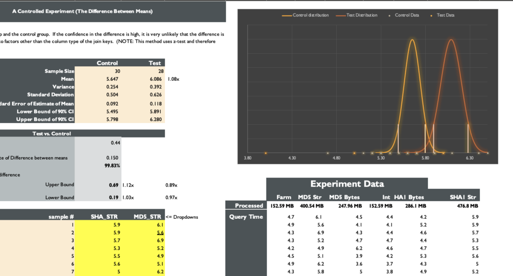
| SHA1 String | MD5 String | 0.44 s | 1.08ⅹ | 99.83 |
Conclusion
Here is everything I took away from this experiment.
- Integers are about 1.2x faster than bytes and about 1.4x faster than strings.
- If you have access to FARM_FINGERPRINT and you’re only using BigQuery, go ahead and use that (you can always switch it up later)
- Otherwise, simply use MD5 as your hash function stored as bytes.
- If you choose to use a string, don’t use hex encoding as I did. Base64 encoding will result in smaller strings and thus faster query times than this (but not as fast as raw bytes)
I’ve made my entire experiment available for you to download in an Excel sheet. I’ve made it dead simple to use. Feel free to add your own data to it and experiment on the data warehouse of your choice!
Click To Download The Experiment Sheet