There is a class of metrics where you simply want to know “How many of thing X are there in total?” but it is utterly impractical to actually count them because there are too many of them to count, or the space over which you’re measuring is too sparse.
Consider the following measurements:
- Number of homeless people in a city
- Number of endangered species in the wild
- Number of illicit drug users
There’s no doubt that quantifying these values is useful in understanding the scope of a problem and devising an effective plan to deal with it.
These questions can all be answered using a clever sampling technique called Mark-Recapture or Capture-Recapture.
In this post, I’m going to show you a simple way you can do this yourself with a simple example.
Let’s Go Fishing
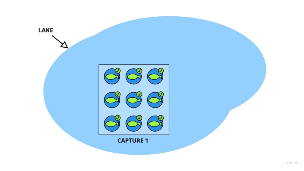
Consider we’re trying to estimate the number of fish in a lake.
We’re going to take our net aboard the boat and go somewhere in the lake and catch 1,000 fish.
Next, we tag the fish with a marker. A permanent marker will do.
Here’s an illustration. I hope you’re not here for the art.
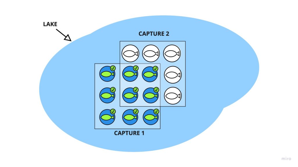
A week later, we come back, and we go somewhere else in the lake. By now, the fish have all scattered around. To keep things simple, we’ll assume the fish generally roam around the whole lake instead of clustering around the shoreline.
We pull up the net and catch another 1200 fish. This time, we look in our net and see 50 fish that already have the mark!
Now, we have everything we need to calculate the total number of fish in the lake! How? Let’s think about it.
The Simple Solution
If 50 of 1,200 fish are marked, that means we’ve marked
50/1200 = 4.16667% <-- Ratio of marked fish in the lake
We had originally marked 1,000 fish, which was 4.16667% of the lake’s total fish. All we have to do is divide by the proportion to get the total population size.
Total # of fish = 1000/4.16667% = 24,000
That wasn’t too hard, was it? It even has a fancy name! This type of estimator is called the Lincon-Peterson estimator and is great when your sample size is big enough.
What this tells you is the expected value or mean of the distribution of potential population size. In other words, due to the effects of randomness, the actual population size may be higher or lower.
“How much higher, or lower,” you ask? To answer this, we need to step it up a notch.
The Robust Solution
We want to know how much uncertainty is really associated with our estimate. There are many ways to calculate this, and Wikipedia gives you a few options, like calculating the confidence interval using an approximation to the normal distribution.
I want to keep things very practical. I always turn to the Beta distribution in situations like this because it comes with a simple and intuitive interpretation that makes it ideal for estimating proportions.
The beta distribution can be thought of as a probability distribution of the percentage of hits in a sample. All we need to know are the number of hits and misses. A hit can be a customer liking our product or, in our case, the existence of a mark on the recaptured fish.
There are 2 parameters, α, and β that define how the Beta distribution will look. For our and purposes, we can think of α=Hits+1 and β=Misses+1.
For example, if we caught 100 fish and 10 of them were marked, we have 10 hits (α = 11) and 90 misses (β = 91), and our probability density function for the beta distribution would look like this:
We had a 10% hit rate, so the bump we expected to see around 0.1 makes sense.
We’d also expect the distribution to be wider if we had a smaller sample, say 1 hit and 9 misses (still a 10% proportion, but now we’re less certain of the true value of the population proportion).
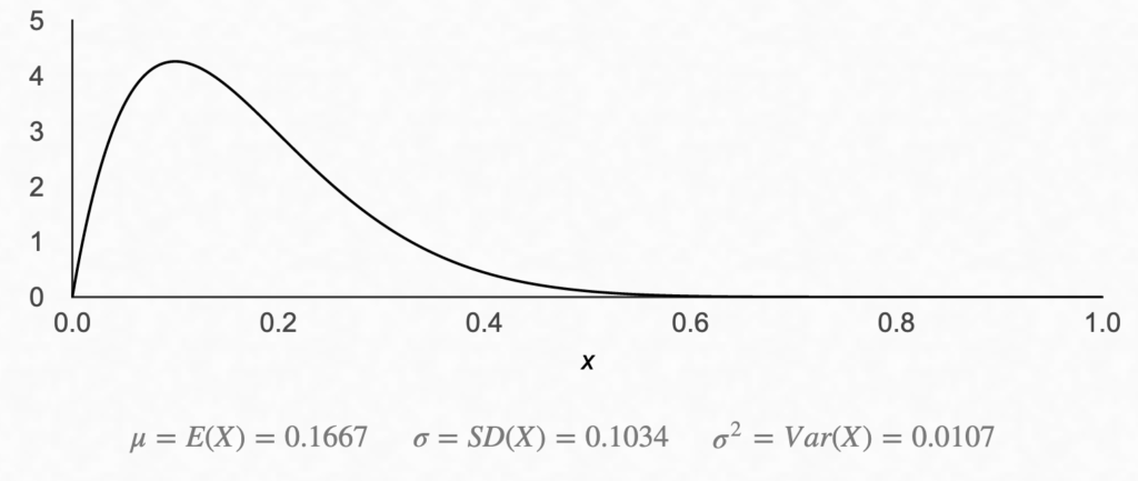
As you can see, there is still a bump around 0.1, but there is a much higher level of uncertainty here… In fact, it seems the real proportion is almost just as likely to be 20% as it is to be 10%.
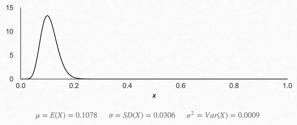
Now, let’s see what our fish example looks like. With our recaptured fish, we had 50 marked out of 1,200 fish. Equivalently, we can say we had 50 hits and 1200 – 50 = 1,150 misses. Add 1 to each, and we have our α and β.
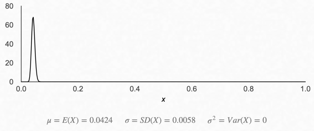
Not too exciting… As we expected, a peak at around 4.17%, but now that we have the distribution, we can calculate the range of potential outcomes.
I want to know the 90% confidence interval. In other words, I want to know the upper bound and lower bound proportions, where 5% of the time, the true population proportion of marked fish falls above the upper bound, and 5% of the time, the value would fall below the lower bound.
To calculate the upper bound, I can equivalently try to find the point x at which P(Fish Marked < x) = 0.95. You can do this with excel using the following formula:
=BETA.INV(0.95, 51, 1151) = 5.24% <-- 90% CI Upper Bound
Similarly, to calculate the lower bound, I can get the point x, at which P(Fish Marked < 5) < 0.05. In excel this would be:
=BETA.INV(0.05, 51, 1151) = 3.33% <-- 90% CI Lower Bound
Now that we have our lower and upper bounds, we can divide 1,200 by each value to get the upper and lower bounds for the total number of fish.
Upper Bound = 1,200/0.0524 = 30,010
Lower Bound = 1,200/0.0333 = 19,083
That seems like a big range, but think about how much you’ve reduced your uncertainty about the number of fish in the lake!
You can always get a better estimate by taking larger samples or taking more samples, but in most cases, having a range may be good enough for you to make a meaningful decision.
Remember… Measurement is not, and has never been, about exact values. Every measurement device is limited in some way.
Conclusion
Counting the fish in a lake may be useless to you, but keep your eyes peeled for real-world cases where you might need to quantify some hidden value, like the number of escaped defects in a manufacturing setting or foot traffic for physical retail stores.
For example, if you’re in a software team, you can split up 2 teams to find bugs in the codebase. The overlap in bugs between teams A and B can be used to calculate total bugs.
Get creative with it and have some fun!
If you find a cool application for this technique, leave a comment, and share your story with others!